Introduction

Spectroscopy datasets often consist of high-dimensional measurements across different wavelengths or wavenumbers, structured in wide-format tables where each column represents a sample and each row corresponds to a spectral position. The tidyspec package provides a tidyverse-friendly toolkit designed to streamline the processing, visualization, and analysis of such spectral data in R.

By building on top of the dplyr, ggplot2, and tidyr ecosystems, tidyspec simplifies common workflows such as baseline correction, unit conversion, normalization, filtering, and principal component analysis (PCA). It enforces consistent treatment of spectral dimensions using a customizable reference column (typically wavenumber or wavelength), which can be easily set using set_spec_wn().

This vignette demonstrates a typical usage of the package, from importing and visualizing spectral data to performing PCA and interpreting results. The functions included are designed to make spectral analysis in R more transparent, reproducible, and user-friendly for both beginners and advanced users.

Instalation

remotes::install_github("marceelrf/tidyspec")

Package overview

The package organizes utilities into 6 families, all prefixed with spec_:

1. Transformation
spec_abs2trans(): Convert absorbance to transmittance. spec_trans2abs(): Convert transmittance to absorbance.

2. Normalization
spec_norm_01(): Normalize spectra to range [0, 1]. spec_norm_minmax(): Normalize to a custom range. spec_norm_var(): Scale to standard deviation = 1.

3. Baseline Correction
spec_blc_rollingBall(): Correct baseline using rolling ball algorithm. spec_blc_irls(): Correct using Iterative Restricted Least Squares. spec_bl_*(): Return baseline vectors (e.g., spec_bl_rollingBall).

4. Smoothing
spec_smooth_avg(): Smooth with moving average. spec_smooth_sga(): Smooth using Savitzky-Golay.

5. Derivative
spec_diff(): Compute spectral derivatives.

6. Preview & I/O
spec_smartplot(): Static preview of spectra. spec_smartplotly(): Interactive preview ({Plotly}). spec_read(): Import from .csv, .txt, .xlsx, etc.

library(tidyspec)
library(tidyverse)

Data

The CoHAspec dataset is a spectral table in wide format, where:

Rows: Wavenumbers (in cm⁻¹).

Columns: Samples (CoHA01, CoHA025, CoHA05, CoHA100).

Values: Absorbance/intensity measurements.

Here’s a preview of the data:

CoHAspec
#> # A tibble: 1,868 × 5
#>    Wavenumber CoHA01 CoHA025 CoHA05 CoHA100
#>         <dbl>  <dbl>   <dbl>  <dbl>   <dbl>
#>  1       399.  0.871   1.36   1.17    1.05 
#>  2       401.  0.893   1.24   1.05    0.925
#>  3       403.  0.910   1.20   0.997   0.876
#>  4       405.  0.914   1.19   0.982   0.867
#>  5       407.  0.908   1.18   0.965   0.857
#>  6       409.  0.887   1.14   0.936   0.828
#>  7       411.  0.856   1.08   0.902   0.791
#>  8       413.  0.819   1.03   0.865   0.748
#>  9       415.  0.789   0.988  0.838   0.717
#> 10       417.  0.768   1.000  0.860   0.735
#> # ℹ 1,858 more rows

Wavenumber Handling

The function set_spec_wn simplifies the use of functions by globally defining the column that contains the wave numbers. User can check the wavenumber column with check_wn_col.

set_spec_wn("Wavenumber")
#> Successfully set 'Wavenumber' as the default wavenumber column.
check_wn_col()
#> The current wavenumber column is: Wavenumber

Visualize the data

Scientists who work with spectroscopy data always want to visualize it after each operation. That’s why we created the spec_smartplot and spec_smartplotly functions to help users.

spec_smartplot creates a static visualization of the spectra, while spec_smartplotly creates an interactive visualization, allowing the user to navigate through the values of the different data.

spec_smartplot(CoHAspec)
#> Warning: wn_col not specified. Using default value: Wavenumber.
#> This message is shown at most once every 2 hours.
#> Warning: xmin not specified. Using default value: 399.1992.
#> This message is shown at most once every 2 hours.
#> Warning: xmax not specified. Using default value: 3999.706.
#> This message is shown at most once every 2 hours.

Static spectral plot showing all samples

spec_smartplotly(CoHAspec,geom = "line")

These functions simplify the process by automating it, but we invite users to make their own figures for presentations and publications. As part of the efforts to create a community of tidyspec users, we plan to create a ggplot2 extension for high-level spectroscopy graphics. For now, you can produce ggplot2 graphs by pivoting the data:

CoHAspec %>% 
  tidyr::pivot_longer(cols = -Wavenumber,
                      names_to = "spectrums",
                      values_to = "absorbance") %>% 
  ggplot(aes(x = Wavenumber, y = absorbance, col = spectrums)) +
  geom_line() #<------ Customize your data from here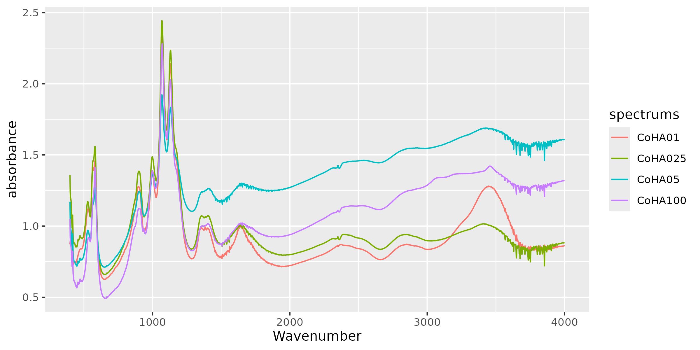

Custom ggplot2 visualization of spectral data

Convert to transmittance (and back to absorbance)

The functions spec_abs2trans and spec_trans2abs are designed to easily convert the spectras.

CoHAspec %>% 
    spec_abs2trans() %>%
    spec_smartplot()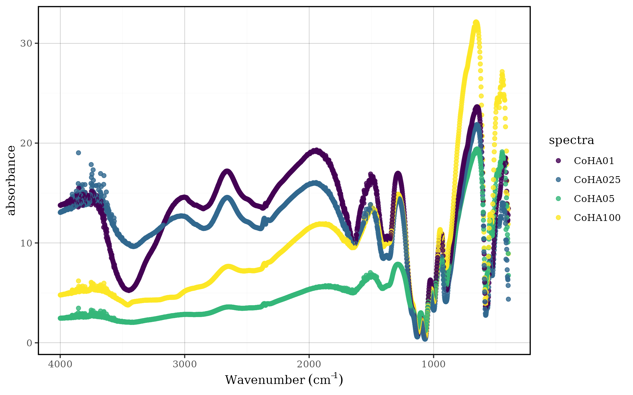

CoHAspec %>% 
    spec_abs2trans() %>%
    spec_trans2abs() %>%
    spec_smartplot()

Select spectra

Tidyspec is designed to be easily integrated with the entire tidyverse ecosystem. Then the user can easily choose which spectra to keep/discard using dplyr::select.

CoHAspec %>% 
    dplyr::select(Wavenumber,CoHA100) %>%
    tidyspec::spec_smartplot()

However, since tidyspec needs the column containing the wave numbers and the user could end up messing up and not keeping it during operations, we decided to develop spec_select which simplifies the process.

CoHAspec %>% 
    tidyspec::spec_select(CoHA100) %>%
    tidyspec::spec_smartplot()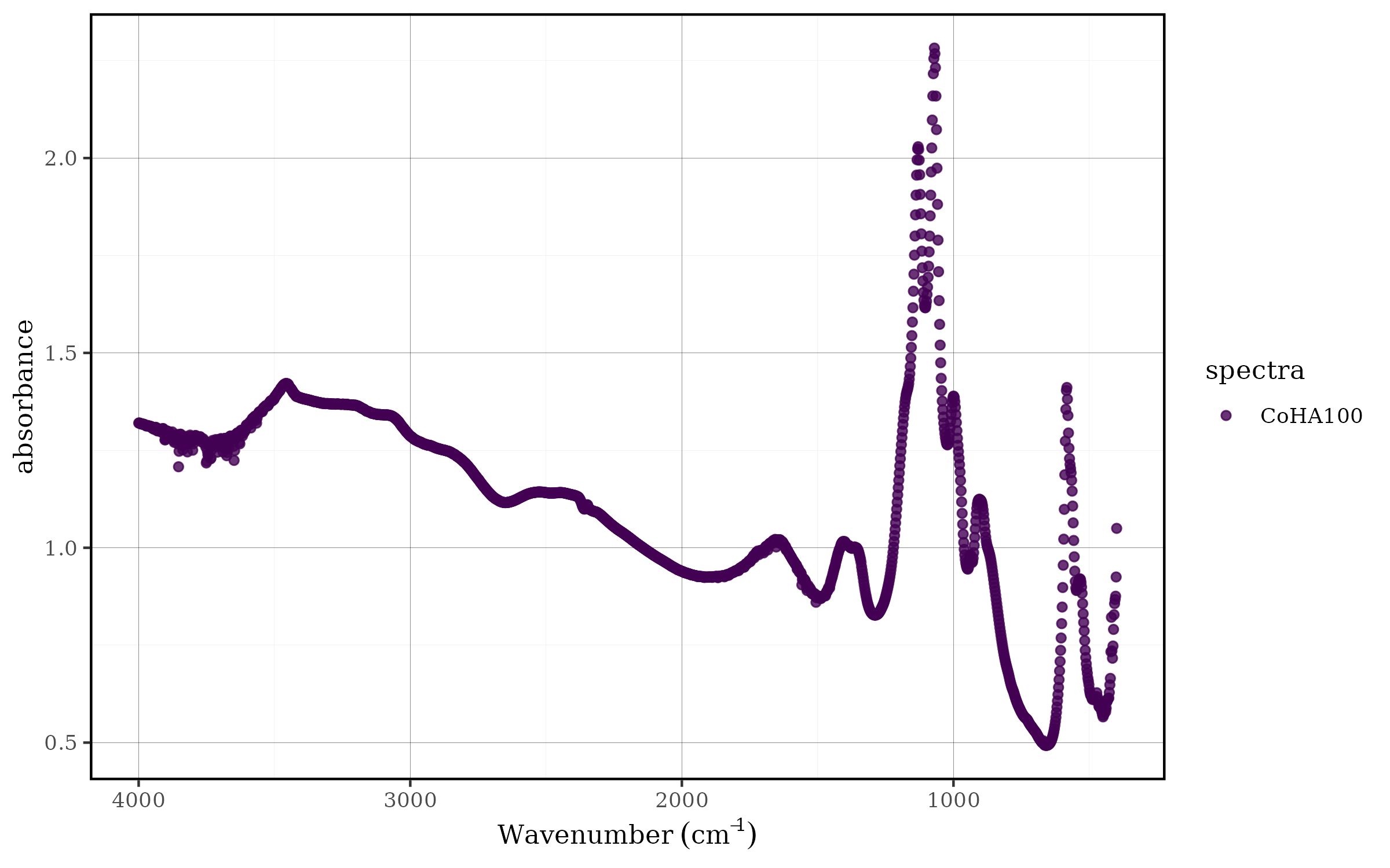

Filter spectra

Similarly to the spectrum selection process, filtering regions of the spectrum can be done using dplyr::filter.

CoHAspec_filt <- 
    CoHAspec %>% 
    tidyspec::spec_select(CoHA100) %>%
    dplyr::filter(Wavenumber > 1000,
                Wavenumber < 1950)

spec_filter simplifies the process of filtering the desired regions.

CoHAspec_filt <- 
    CoHAspec %>% 
    spec_select(CoHA100) %>%
    spec_filter(wn_min = 1000,
                wn_max = 1950)

spec_smartplot(CoHAspec_filt, geom = "line")

With `spec_select`

Smoothing the data

Spectroscopic data often contains noise that can interfere with analysis and interpretation. Smoothing techniques help reduce this noise while preserving the essential spectral features. The tidyspec package provides two main smoothing methods: moving averages and Savitzky-Golay filtering.

Moving averages method

The moving average method (spec_smooth_avg()) is one of the simplest and most intuitive smoothing techniques. It works by replacing each data point with the average of its neighboring points within a specified window size. This method is particularly effective for reducing random noise while maintaining the overall shape of spectral peaks.

How it works:

For each point, it calculates the mean of surrounding points within a defined window
Larger windows provide more smoothing but may blur important features
Smaller windows preserve detail but provide less noise reduction

Parameters:

wn_col: Column name for wavelength data (default: “Wn”)
window: Window size for the moving average (default: 15)
degree: Polynomial degree for smoothing (default: 2)

CoHAspec_filt %>% 
  spec_smooth_avg() %>%
  spec_smartplot(geom = "line")

Savitz-Golay method

The Savitzky-Golay filter (spec_smooth_sga()) is a more sophisticated smoothing technique that is particularly well-suited for spectroscopic data. Unlike simple moving averages, this method fits a polynomial to a local subset of data points and uses this polynomial to estimate the smoothed value. This approach is especially effective at preserving peak shapes, heights, and widths while reducing noise.

How it works:

For each data point, it fits a polynomial of specified degree to nearby points within a window
The smoothed value is calculated from this local polynomial fit
This preserves the underlying spectral features better than simple averaging
The method can also calculate derivatives directly during the smoothing process

Parameters:

wn_col: Column name for wavelength data (default: “Wn”)
window: Window size for smoothing (default: 15, should be odd)
forder: Polynomial order for fitting (default: 4)
degree: Degree of differentiation (default: 0 = smoothing only)

CoHAspec_filt %>% 
  spec_smooth_sga() %>%
  spec_smartplot(geom = "line")

Comparison with moving average:

Savitzky-Golay: Better peak preservation, more computationally intensive
Moving average: Faster computation, simpler implementation, more peak distortion

Derivatives

Differentiation of spectral data is a fundamental technique in chemometrics that allows for highlighting specific spectral features, reducing baseline effects, and improving the resolution of overlapping peaks. The spec_diff() function implements numerical differentiation for spectral data, offering flexibility to calculate first-order or higher-order derivatives.

Using the `spec_diff()` Function

The spec_diff() function accepts the following arguments:

.data: A data.frame or tibble containing spectral data
wn_col: A character string specifying the column name for the wavelength data (default: “Wn”)
degree: A numeric value specifying the degree of differentiation. If degree = 0, the original data is returned without any changes

Example:

CoHAspec_filt %>% 
    tidyspec::spec_smooth_sga() %>%
    spec_diff(degree = 2) %>%
    tidyspec::spec_smartplot(geom = "line")
#> Warning: Removed 2 rows containing missing values or values outside the scale range
#> (`geom_line()`).

In this pipeline:

The filtered spectral data (CoHAspec_filt) is first smoothed using the Savitzky-Golay algorithm
Then, a second-order derivative is applied using spec_diff(degree = 2)
The result is visualized through spec_smartplot() with line geometry

Baseline correction

Baseline correction is a crucial preprocessing step in spectral analysis that removes systematic variations in the baseline that are not related to the analyte of interest. These baseline variations can arise from instrumental drift, scattering effects, sample positioning, or optical interferences. Proper baseline correction enhances spectral quality and improves the accuracy of subsequent quantitative and qualitative analyses.

Rolling ball method

The rolling ball algorithm is a popular baseline correction technique that estimates the baseline by “rolling” a virtual ball of specified radius beneath the spectrum. This method is particularly effective for correcting baselines with smooth, curved variations and is widely used in various spectroscopic applications.

Function Parameters

The spec_blc_rollingBall() function provides comprehensive control over the baseline correction process:

.data: A data.frame or tibble containing spectral data
wn_col: Column name for wavelength data (default: “Wn”)
wn_min: Minimum wavelength for baseline correction range
wn_max: Maximum wavelength for baseline correction range
wm: Window size of the rolling ball algorithm (controls ball radius)
ws: Smoothing factor of the rolling ball algorithm
is_abs: Logical indicating if data is in absorbance format

Baseline Correction Application

The following example demonstrates baseline correction applied to a specific wavelength range:

CoHAspec_filt %>% 
    spec_smooth_sga() %>%
    spec_blc_rollingBall(wn_min = 1030,
                         wn_max = 1285,
                         ws = 10,
                         wm = 50) %>%
    tidyspec::spec_smartplot(geom = "line")

In this pipeline:

Smoothing is applied first to reduce noise
Rolling ball correction is performed in the 1030-1285 cm⁻¹ range
Window size (wm = 50) and smoothing factor (ws = 10) are optimized for the data

Looking to the baseline

To better understand the correction process, we can examine the estimated baseline using spec_bl_rollingBall():

CoHAspec_filt %>% 
    spec_smooth_sga() %>%
    spec_bl_rollingBall(wn_col = "Wavenumber",
                        wn_min = 1030,
                        wn_max = 1285,
                        ws = 10,
                        wm = 50) %>% 
  spec_smartplot()

This visualization shows only the estimated baseline, allowing you to assess whether the algorithm properly captures the underlying baseline trend.

Comparing Original and Baseline

For a comprehensive view of the correction process, we can overlay the original spectrum with the estimated baseline:

bl <- CoHAspec_filt %>% 
    spec_smooth_sga() %>%
    spec_bl_rollingBall(wn_col = "Wavenumber",
                         wn_min = 1030,
                         wn_max = 1285,
                         ws = 10, wm = 50)

CoHAspec_filt %>%
  spec_smooth_sga() %>%
  spec_filter(wn_min = 1030, wn_max = 1285) %>% 
  left_join(bl) %>% 
  spec_smartplot(geom = "line")
#> Joining with `by = join_by(Wavenumber, CoHA100)`

This comparison allows you to:

Evaluate the baseline estimation quality
Identify regions where the algorithm may need parameter adjustment
Verify that the baseline follows the expected spectral trend

Scaling the spectra

Spectral scaling (normalization) is a preprocessing technique that standardizes spectral data to facilitate comparison between samples and improve the performance of multivariate analysis methods. Different scaling approaches address various sources of systematic variation in spectral data, such as differences in sample concentration, path length, or instrumental response.

Importance of Spectral Scaling

Scaling is essential when:

_ Sample concentrations vary: Different analyte concentrations can mask spectral patterns _ Path lengths differ: Variations in sample thickness affect overall intensity _ Instrumental variations exist: Different measurement conditions create systematic offsets _ Multivariate analysis is planned: Many chemometric methods assume standardized data _ Pattern recognition is the goal: Scaling emphasizes spectral shape over absolute intensity

Working with a Spectral Region

For demonstration purposes, we’ll work with a specific spectral region that contains relevant analytical information:

CoHAspec_region <- CoHAspec  %>%
    dplyr::filter(Wavenumber > 1300,
                Wavenumber < 1950) 
CoHAspec_region %>% 
    spec_smartplot(geom = "line")

This region (1300-1950 cm⁻¹) is selected to focus on specific spectral features while avoiding regions that might contain noise or irrelevant information.

Min-Max Normalization (0-1 Scaling)

Min-max normalization scales each spectrum to a range between 0 and 1, preserving the relative relationships between spectral intensities while standardizing the dynamic range.

Mathematical Foundation

For each spectrum, the transformation is:

Normalized value = (Value - Minimum) / (Maximum - Minimum)
Results in values ranging from 0 to 1
Preserves the original spectral shape

CoHAspec_region %>%
    spec_norm_01() %>% 
    spec_smartplot(geom = "line")

The spec_norm_01() function:

Finds the minimum and maximum values for each spectrum
Applies the min-max transformation
Maintains spectral shape while standardizing intensity range
Is particularly useful when absolute intensity differences are not analytically relevant

When to Use Min-Max Normalization

Min-max scaling is ideal when:

You want to preserve spectral shape
Absolute intensities vary due to concentration differences
Visual comparison of spectral patterns is important
The dynamic range needs standardization

The user can set any min and max value with the spec_norm_minmax() function:

CoHAspec_region %>%
    spec_norm_minmax(min = 1, max = 2) %>% 
    spec_smartplot(geom = "line")

Standardization (Z-score Normalization)

Standardization transforms each spectrum to have a mean of 0 and standard deviation of 1, emphasizing deviations from the average spectral response.

Mathematical Foundation

For each spectrum, the transformation is:

Standardized value = (Value - Mean) / Standard Deviation
Results in mean = 0 and variance = 1
Emphasizes relative variations around the mean

Application

CoHAspec_region %>%
    spec_norm_var() %>% 
    spec_smartplot(geom = "line")

The spec_norm_var() function:

Calculates the mean and standard deviation for each spectrum
Applies z-score transformation
Centers the data around zero
Standardizes the variance across all spectra

When to Use Standardization

Standardization is appropriate when:

You want to emphasize spectral variations
Baseline shifts need to be removed
Multivariate analysis requires standardized inputs
Focus is on relative changes rather than absolute values

Choosing the Right Scaling Method

The choice between scaling methods depends on your analytical objectives:

Method	Best for	Preserves	Emphasizes
Min-Max (0-1)	Pattern recognition, visual comparison	Spectral shape	Relative intensities
Standardization	Multivariate analysis, variance-based methods	Spectral variations	Deviations from mean

Integration with tidyverse

One of the key strengths of tidyspec is its seamless integration with the tidyverse ecosystem. This design philosophy allows users to leverage the full power of dplyr, tidyr, purrr, and other tidyverse packages to create sophisticated spectral analysis workflows. The following examples demonstrate how to combine tidyspec functions with tidyverse tools to solve common analytical challenges.

Case 1: Choosing the best baseline parameters

Parameter optimization is a critical aspect of spectral preprocessing. The rolling ball baseline correction method has two key parameters: ws (smoothing factor) and wm (window size), and finding the optimal combination often requires systematic evaluation across multiple parameter sets. The tidyverse approach makes this process both elegant and efficient.

Setting up the parameter grid

First, we prepare our spectral data by focusing on a specific region and applying initial smoothing:

dados_1030_1285 <- CoHAspec_filt %>% 
    tidyspec::spec_smooth_sga() %>%
    dplyr::filter(Wavenumber <= 1285, Wavenumber >= 1030)

Next, we create a comprehensive parameter grid using tidyr::crossing(), which generates all possible combinations of the specified parameter values:

params <- tidyr::crossing(ws_val = c(2,4,6,8,10,12),
                          wm_val = c(10, 25, 40, 50))
params 
#> # A tibble: 24 × 2
#>    ws_val wm_val
#>     <dbl>  <dbl>
#>  1      2     10
#>  2      2     25
#>  3      2     40
#>  4      2     50
#>  5      4     10
#>  6      4     25
#>  7      4     40
#>  8      4     50
#>  9      6     10
#> 10      6     25
#> # ℹ 14 more rows

This approach creates a systematic grid of 24 parameter combinations (6 × 4), ensuring thorough exploration of the parameter space.

Applying baseline correction across parameters

The power of the tidyverse becomes evident when we need to apply the same operation across multiple parameter sets. Using dplyr::mutate() with purrr::pmap(), we can efficiently apply baseline correction to each parameter combination:

df <- params %>%
    dplyr::mutate(spectra = list(dados_1030_1285)) %>%
    dplyr::mutate(spectra_blc = purrr::pmap(list(spectra, ws_val, wm_val),
                             \(x, y, z ) spec_blc_rollingBall(.data = x, ws = y, wm = z))) %>%
    dplyr::mutate(title = paste0("ws = ", ws_val," , wm = ", wm_val )) %>%
    dplyr::mutate(plot = purrr::map2(spectra_blc, title, ~ spec_smartplot(
            .data = .x,
            wn_col = "Wavenumber",
            geom = "line") + labs(title = .y)
            ))

This pipeline demonstrates several key tidyverse concepts:

Nested data structures: Each row contains the complete spectral dataset
Functional programming: purrr::pmap() applies the baseline correction function across multiple arguments
Pipeline operations: Each step builds upon the previous one using the pipe operator
Automated visualization: purrr::map2() creates customized plots for each parameter combination

Visualizing parameter optimization results

The final step involves creating comparative visualizations to assess the effect of different parameter combinations:

library(gridExtra)
#> 
#> Attaching package: 'gridExtra'
#> The following object is masked from 'package:dplyr':
#> 
#>     combine

grid.arrange(grobs = df$plot[1:4], nrow = 2, ncol = 2)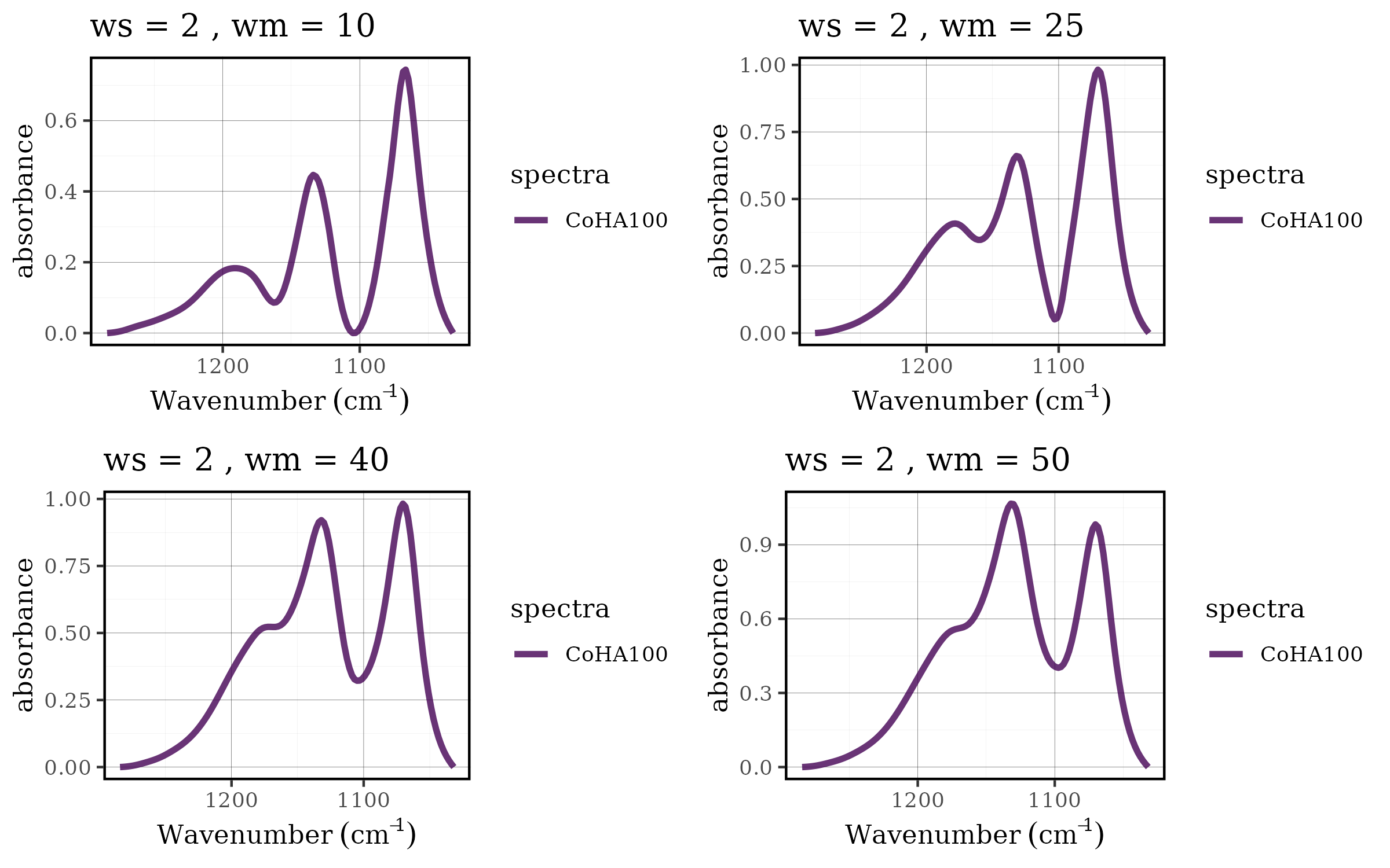

grid.arrange(grobs = df$plot[5:8], nrow = 2, ncol = 2)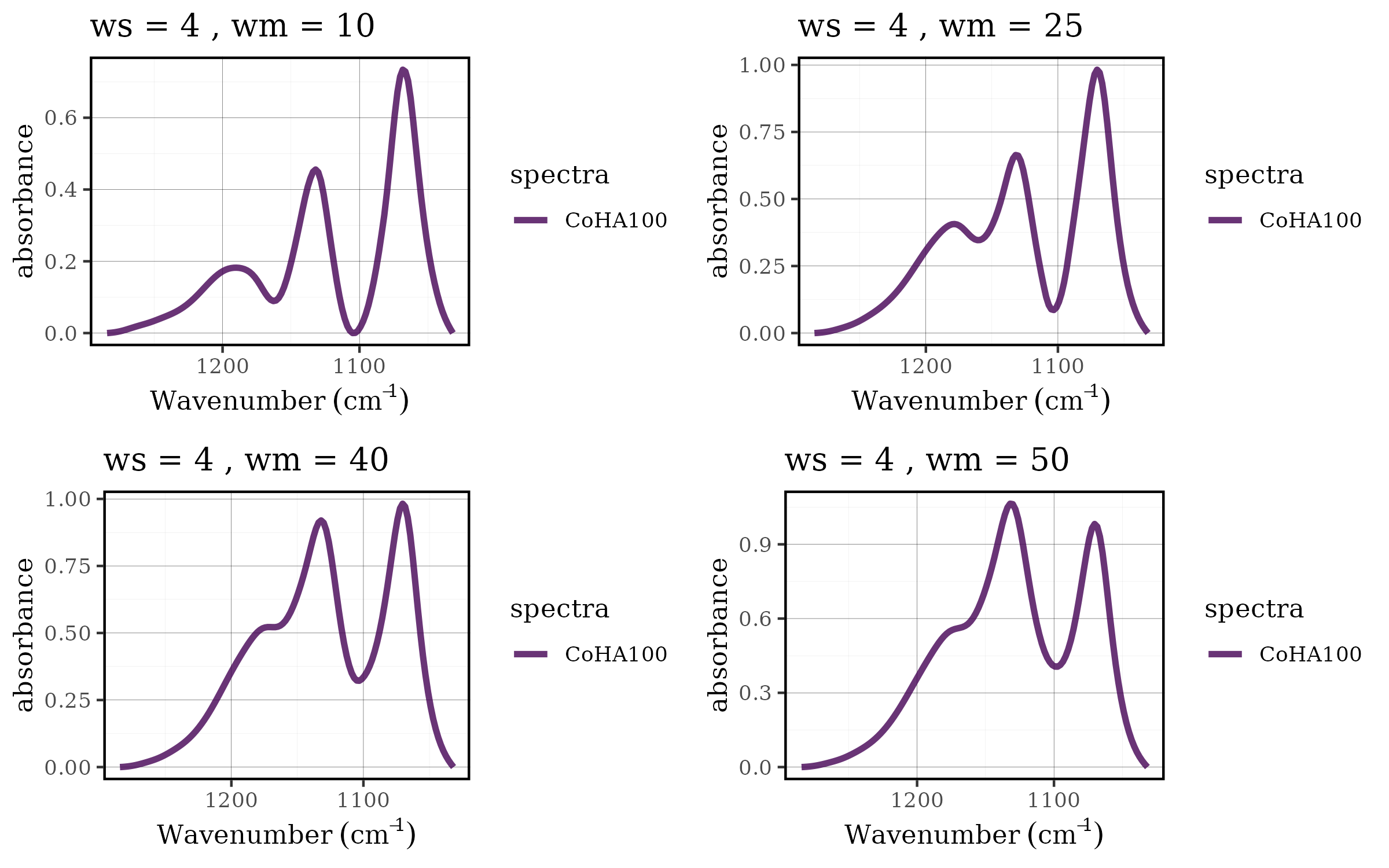

grid.arrange(grobs = df$plot[9:12], nrow = 2, ncol = 2)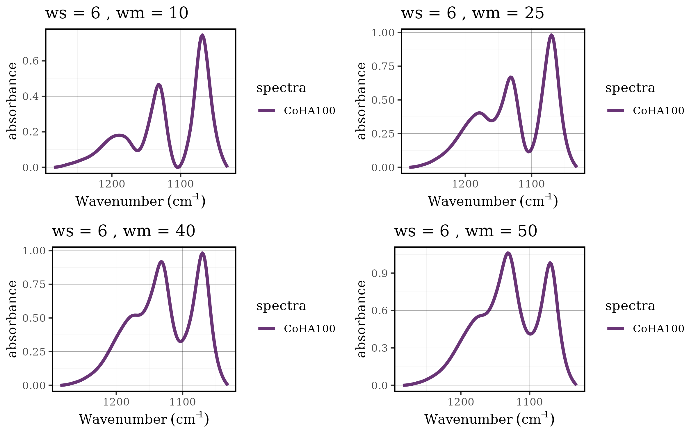

grid.arrange(grobs = df$plot[13:16], nrow = 2, ncol = 2)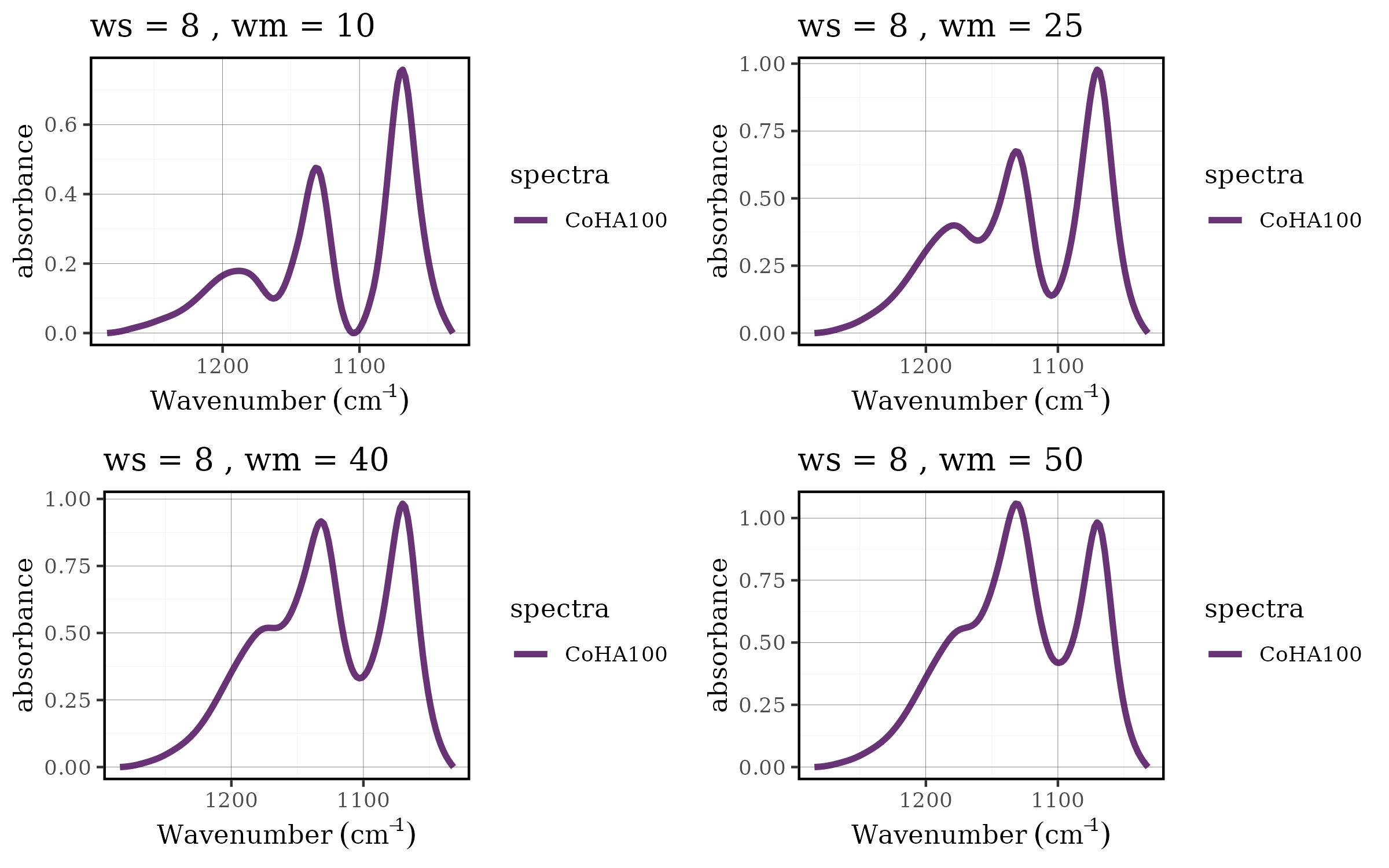

grid.arrange(grobs = df$plot[17:20], nrow = 2, ncol = 2)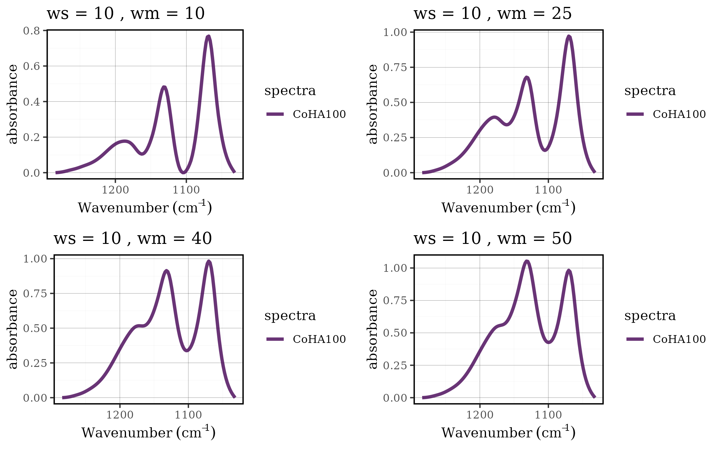

grid.arrange(grobs = df$plot[21:24], nrow = 2, ncol = 2)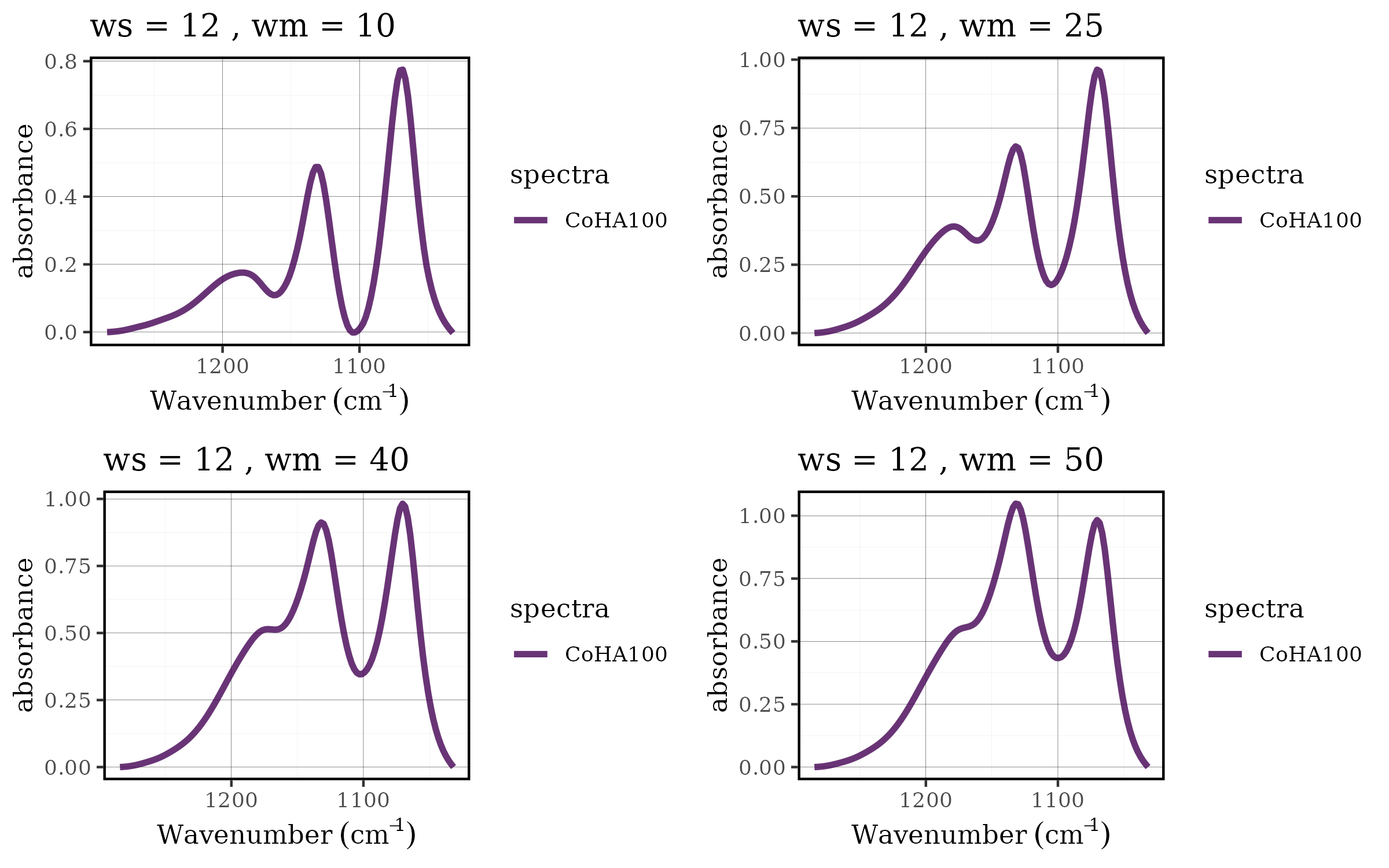

Benefits of the tidyverse approach

This workflow demonstrates several advantages of integrating tidyspec with the tidyverse:

Scalability: Easy to add more parameters or parameter values
Reproducibility: All steps are clearly documented and can be easily modified
Efficiency: Vectorized operations handle multiple datasets simultaneously
Flexibility: Each step can be customized or extended as needed
Readability: The pipeline structure makes the analysis workflow transparent

Extending the approach

This methodology can be extended to optimize other spectral processing parameters:

Smoothing parameters (window size, polynomial order)
Normalization methods and ranges
Derivative calculation parameters Spectral filtering ranges

The combination of tidyspec functions with tidyverse tools creates a powerful framework for systematic spectral analysis, enabling researchers to make data-driven decisions about preprocessing parameters while maintaining clean, reproducible code.

Instalation

Package overview

Data

Wavenumber Handling

Visualize the data

Convert to transmittance (and back to absorbance)

Select spectra

Filter spectra

Smoothing the data

Moving averages method

How it works:

Parameters:

Savitz-Golay method

How it works:

Parameters:

Comparison with moving average:

Derivatives

Using the spec_diff() Function

Baseline correction

Rolling ball method

Function Parameters

Baseline Correction Application

Looking to the baseline

Comparing Original and Baseline

Scaling the spectra

Importance of Spectral Scaling

Working with a Spectral Region

Min-Max Normalization (0-1 Scaling)

Mathematical Foundation

When to Use Min-Max Normalization

Standardization (Z-score Normalization)

Mathematical Foundation

Application

When to Use Standardization

Choosing the Right Scaling Method

Integration with tidyverse

Case 1: Choosing the best baseline parameters

Setting up the parameter grid

Applying baseline correction across parameters

Visualizing parameter optimization results

Benefits of the tidyverse approach

Extending the approach

Using the `spec_diff()` Function